The Feigenbaum Tree is the “bifurcation” graph of iterating the function:
f_r(y) = 4 r y (1-y)
r is a constant, 0.25 < r < 1
and
0 ≤ y ≤ 1
The iteration of f defines a sequence:
y1 = f_r(y0) (1st iteration)
y2 = f_r(y1) (2nd iteration)
y3 = f_r(y2) (3rd iteration)
…
We want to find out the behavior of the sequence. (with different values of r, and different initial value y0.)
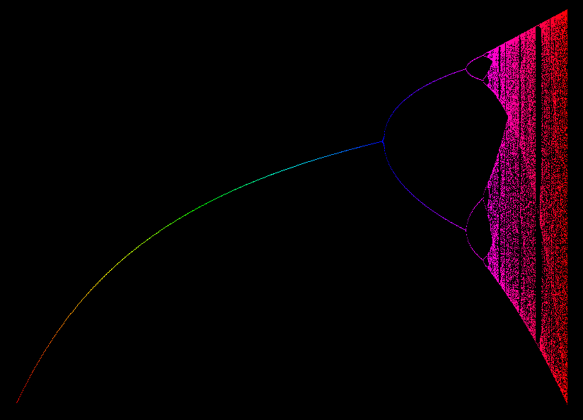
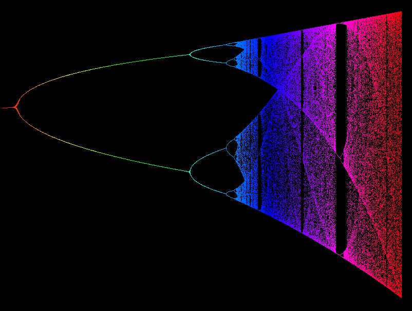
Feigenbaum Tree
The horizontal axes represents the values of constant r, from 1/4 to 1 . So, each vertical line represents a specific function f.
The vertical axes range from 0 to 1, representing the values of f's iteration sequence.
Each dot is a value f, from 1000 to 2000 iterations.
From this graph we see, that when r is small (e.g. r=1/4), iteration sequence converges to a single value. When r is a bit larger, it hops around 2 values (said to have orbit of 2). As r gets larger, the iteration of f exhibit chaotic behavior.
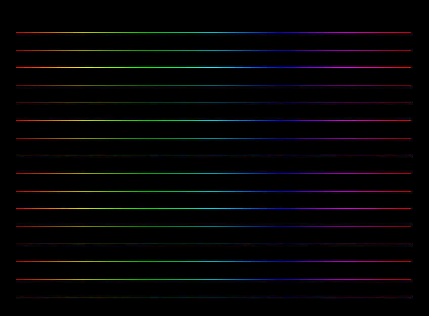
Feigenbaum Tree, 16 initial values, 0th iteration.
The horizontal axes represent values of the constant r, from 0.25 to 1.
The vertical axes represent 16 initial values, evenly distributed, from 0 to 1.
(Points of the same color represent the same value of r.)
16 initial values after 6 iterations.
Look at the left edge, where r=1/4. After 6 iterations, 16 initial values all got closer, converging around 0.2.
Look at the middle, the blue colored section, when r is around 0.7. Different initial values y0 also ends up closer, converging around 0.5.
Look at the right, when r=1, evenly distributed initial values of f are now scattered after 6 iterations.
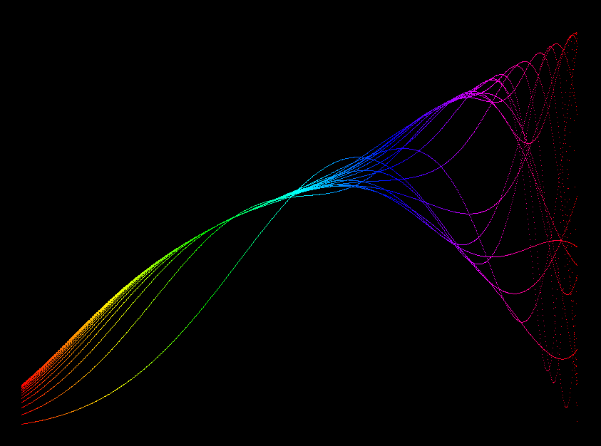
after 20 iterations
After 20 iterations this picture evolved. Roughly up to r = 0.75 all iterated points
lie on one curve, the fixed points of the map, obtained from y = 4 r*y(1-y) or, for y not 0,
1 = 4 r (1-y) with solution y = (4 r - 1)/(4 r). For r < 0.75 the derivative of f_a (that is
f'(y) = 4 r *(1-2 y) at the fixed point has absolute value < 1, therefore the fixed point
is attracting all other points (= the distance to the fixed point gets smaller under each
iteration).
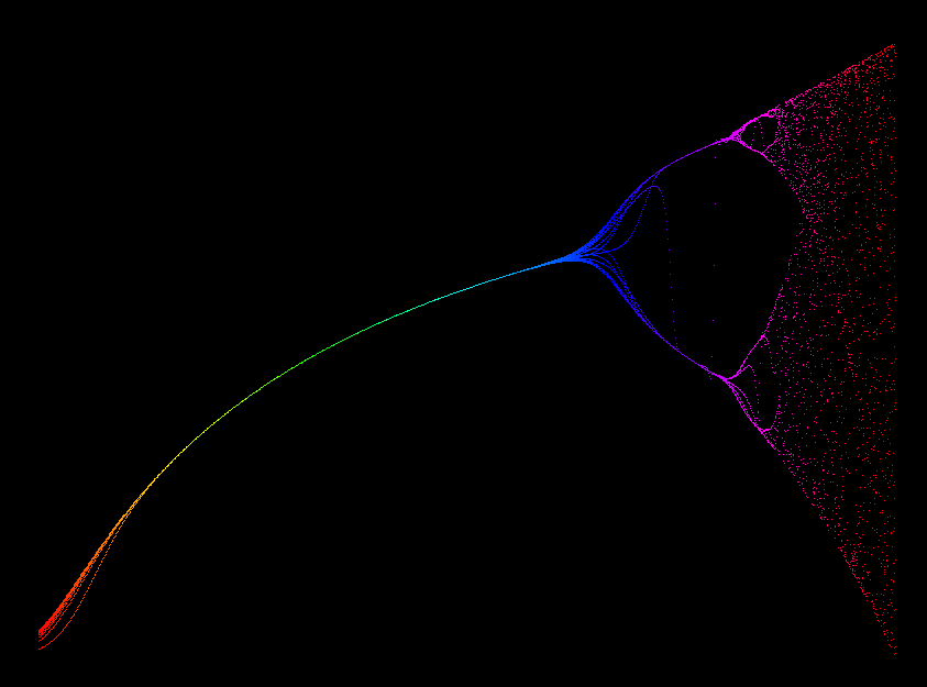
Feigenbaum Tree 0.25 1
After several 100 iterations this picture is obtained. What does the branching of the
fixed point curve into 2 branches mean? We enlarge the picture.
Feigenbaum Tree 0.74 1
In this image the simple part of the Feigenbaum Tree is left away and the part for 0.7 < r < 1
is stretched over the full screen. We see that there is more branching initially and more thinned
out parts for larger parameter r.
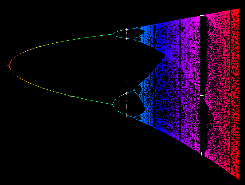
Feigenbaum orbits
We added the iteration of three points into the previous picture. Recall, that the y-points
are iterated in the vertical direction, because they belong to the same r value. The starting
point in the three cases is, more or less, the point in the middle of that vertical line.
The iterated points keep approaching the branches of the tree. So, for the green parameter
the iterated white points converge to an orbit of period 2. In the cyan range the whitepoints
converge to an orbit of period 4. In the magenta range the white points converge to an orbit
of period 3.
The densely populated parts in between are called “chaotic regions”.
And what do the thick curves in the chaotic parts signify? Clearly there were more of our
iterated points near the thick curves than where the dot pattern is thinner. We discretize
the y-space into pixel-sized points and count, how often these pixelpoints are visited:
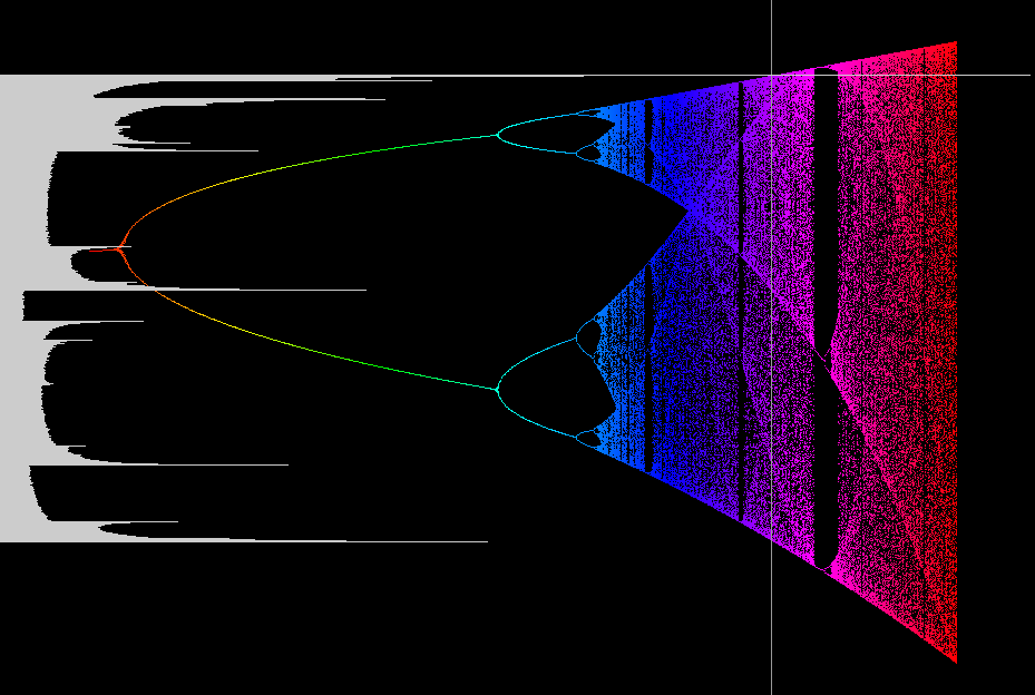
Feigenbaum visibility count
The vertical white line says which r-value was selected. All the pixels between y = 0
and y = 1 are iterated. After a few hundred iterations we start to count how often a pixel
is visited. For each initial pixel we plot, horizontally in white, how often this pixel
has been visited. The highest spikes of this plot indeed are exactly where the thick curves
are in tree at the selected value r (vertical white line). Our white plot is therefore a
density plot for the iteration with the chosen r value.