In the same way as we can get an impression of the earth by studying charts, we can understand
hyperbolic geometry by viewing the unit disk as a chart. An essential information for charts is
their scale. The scale for our hyperbolic chart is this: For any curve c(t) in the unit disk
the hyperbolic length ||c'(t)|| of its tangent vectors is a multiple of its euclidean length |c'(t)|:
||c'(t)||^2 = |c'(t)|^2 / (1 - |c(t)|^2).
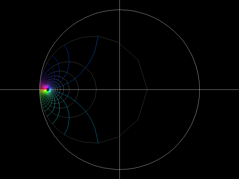
hyperbolic transl 001
map: z ⟶ f(z) = (z + c) / (1 + con(c)*z), domain: polar grid 0.1 < |z| < 0.95,
morph -0.9 < c < 0.9, range: unit disk.
All these Moebius transformations map the unit disk to itsself. They are compatible with the
hyperbolic chart scale: The hyperbolic length of a tangent vector of a curve and its image under
these Moebius transformations have the same hyperbolic length.
The angular parameter lines are “hyperbolic circles”, meaning: the points of such a circle have all the
same hyperbolic distance from the hyperbolic center of that circle.
The radial parameter lines are hyperbolic “shortest connections” between their endpoints. Such curves are called
“geodesics”. In this case they are circles which meet the unit circle orthogonally.
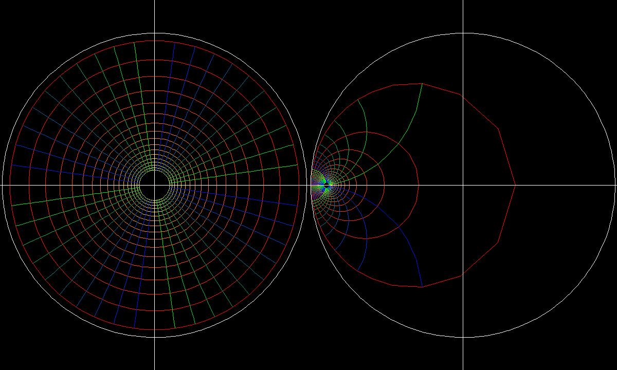
The morph shows a hyperbolic translation along the real axis.
The disk is one model of hyperbolic geometry and what you see
is a family of polar coordinates around points on the real axis.
The movement of “disks” is a visualization of hyperbolic translation.
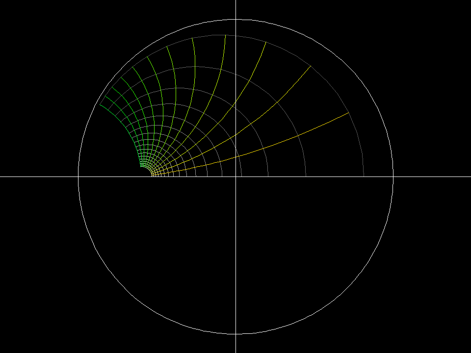
hyperbolic rotation 001
map: z ⟶ f(z) = (z + c) / (1 + con(c)*z), domain: one quarter polar grid 0.1 < |z| < 0.95, angle from 0 to pi/2.
morph: add a*2pi to all angles and morph 0 < a < 1, range: unit disk.
The morph shows a hyperbolic rotation around the hyperbolic center of the polar grid.