z → z^e
with the e varying from 0.5 (square root) to 2 (square),
on rectangular grid.
The
images of the parameter lines are
parabolas for
e = 2,
and hyperbolas for e = 0.5 and e = 1.5.
The white circle is the unit circle. Points on the unit circle are mapped to the unit circle.
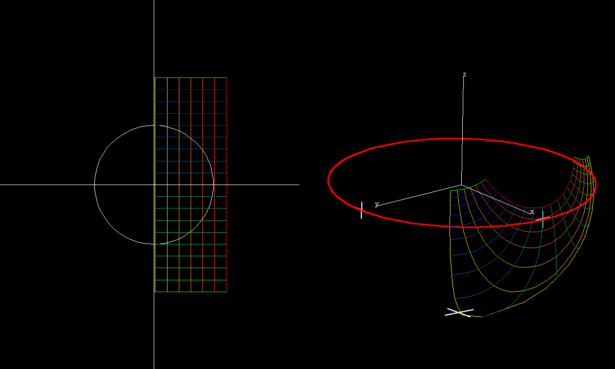
z → z^e, e from 0.5 to 2, on a rectangular grid in the
then stereographically projected to a sphere.
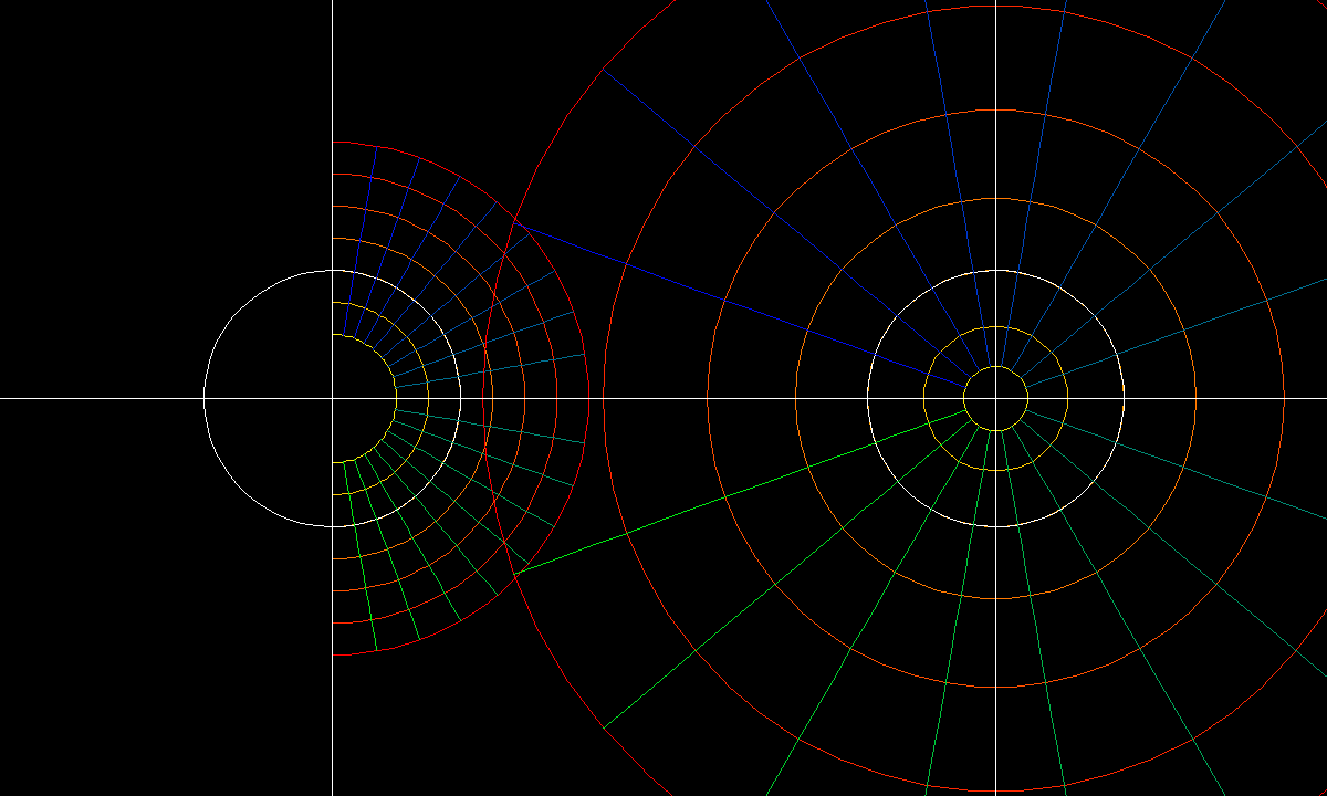
z → z^e with the e varying from 0.5 to 2, on polar grid.
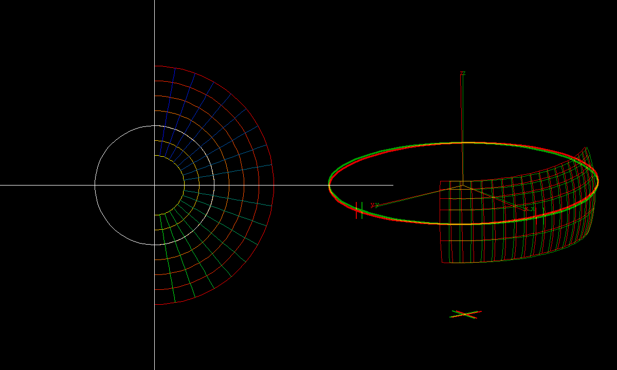
z → z^e with the e varying from 0.5 to 2, on polar grid, then stereographically projected to the sphere. The fat circle is the image of the unit circle, it is the
equator of the Riemann sphere. 0, 1, i are marked by crosses.
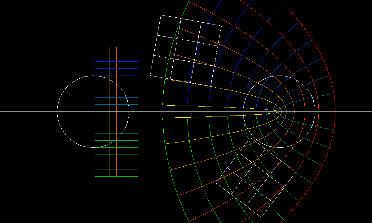
shows the image with two derivative approximations.
Since we visualize complex functions as maps, one should visualize the derivative f'(z0) at a point z0 as the linear map (z - z0) → f(z0) + f'(z0)*(z - z0). We show for two values of z0 the images of this derivative map, applied to a (3 x 3) subgrid of the domain grid (with one vertex at z0).
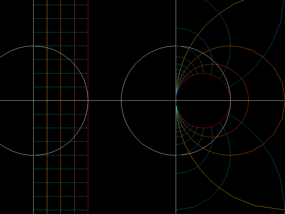
function: z → 1/z
domain: cartesian square grid, 0 ≦ Re(z) ≦ 1, -10 ≦ Im(z) ≦ 10.
range : parameter lines are circles in the Gaussian plane which touch the axes.
The inverse function is used to produce this circle grid in the right half plane.
In the next image the squaring function is applied to this circle grid.
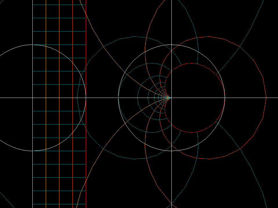
function: z → 1/z^2
domain: cartesian square grid, 0 ≦ Re(z) ≦ 1, -10 ≦ Im(z) ≦ 10.
range : parameter lines are cardioids in the Gaussian plane that touch the x-axis.
Apply the complex squaring function to the previous circle grid in the right half plane.
This two step approach is easier to imagine than applying 1/z^2 to the shown cartesian grid.
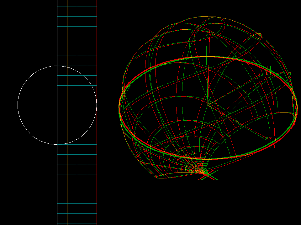
function: z → 1/z
domain: cartesian square grid, 0 ≦ Re(z) ≦ 1, -10 ≦ Im(z) ≦ 10.
range : parameter lines are cardioids shown on the Riemann sphere.