Back to interactive Constant Torsion Curves
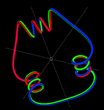
Constant torsion morph
Geometric invariants of curves are easier to explain when the curve is parametrized by arc length.
Then the torsion function of the space curve measures, how fast the second derivative of the curve
rotates around the curve. The animation shows curves of constant torsion for which the curvature
is a trigonometric polynomial. For certain coefficients of the polynomial these curves are closed
curves - there are three of them in this animation.
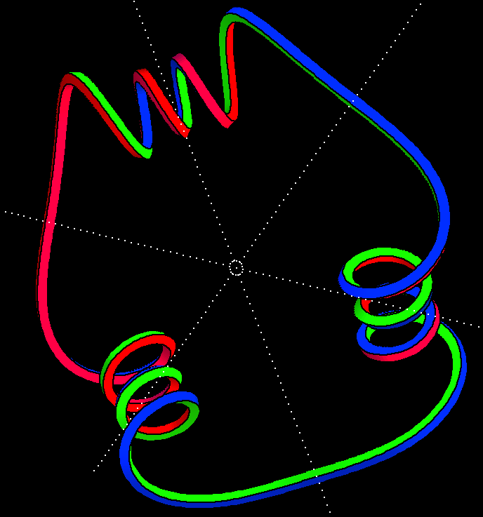
Whether the curve closes or not, we know from the curvature function
for which parameter values 180 degree rotation about the principal normal
of the curve is a symmetry. The construction of closed curves proceeds
in two steps: first we choose parameters so that two neighboring symmetry
normals intersect. Then all symmetry normals pass through this point. Then
the parameters are further restricted so that the angle between neighboring
symmetry normals is a rational number times pi, for 3-fold symmetry we
adjust to pi/3, for 4-fold symmetry we adjust to pi/4.
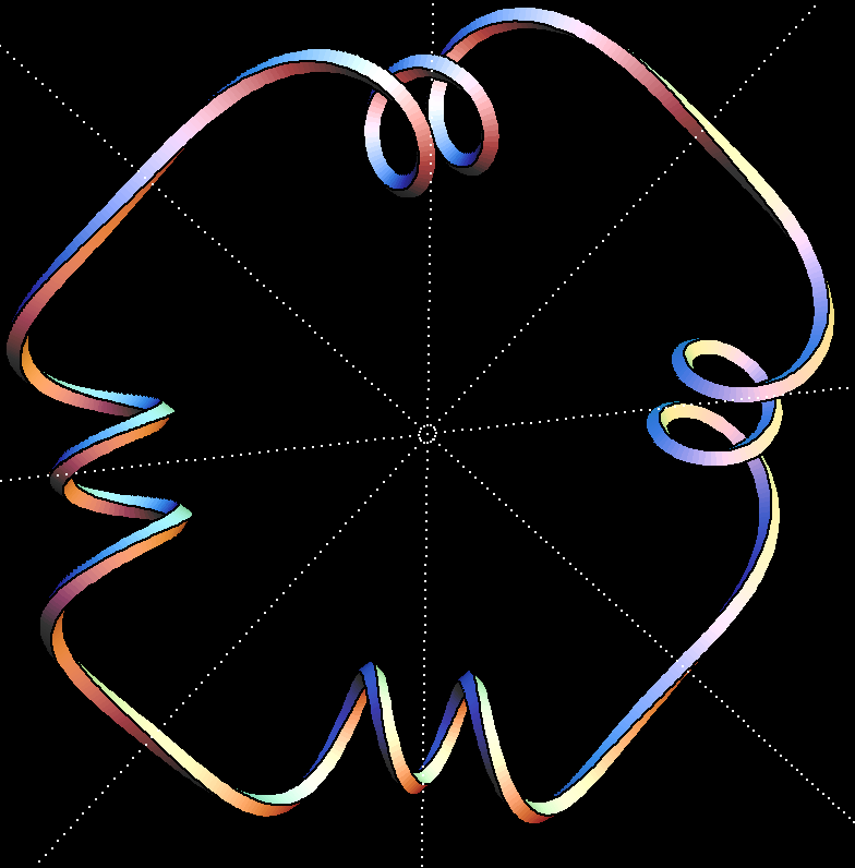
The curvature function changes sign in these examples. This is not allowed for
Frenet curves because the definition of the principal normal fails where the curvature is zero.
This does not hinder the integration of the Frenet ODE, leading to these
analytic curves.
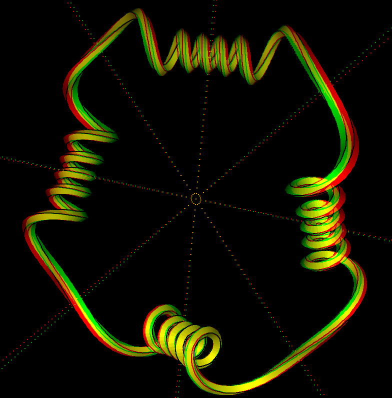
the symmetry of constant torsion examples can easily be changed.
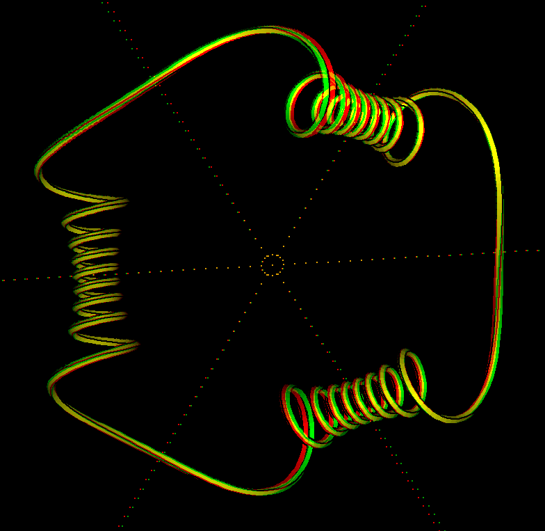
anaglyph example with 3-fold symmetry.
another constant torsion anaglyph.